Manual update loop for more control#

While GLM.stochastic_fit provides a convenient interface for most use cases, in some situations fine-grained manual control during the optimization loop might be required.

As a starting point for more advanced users needing such control, we show how to manually set up a training loop performing stochastic gradient descent (SGD).

Warning

SVRG is particularly suited for stochastic optimization, but its optimization loop is more involved than for SGD, so using GLM.stochastic_fit is highly recommended.

Set up the data and model#

import jax
import matplotlib.pyplot as plt
import numpy as np
import pynapple as nap
import seaborn as sns

import nemos as nmo
from nemos._documentation_utils._stochastic_optim_toy_data import (
    _simulate_batching_data,
)

jax.config.update("jax_enable_x64", True)
nap.nap_config.suppress_conversion_warnings = True
np.random.seed(123)

This approach doesn’t require the use of a NeMoS data loader, you can load batches of data any way you want. Here, we will use in-memory data and ArrayDataLoader for simplicity.

units, spike_trains, X = _simulate_batching_data()

loader = nmo.batching.ArrayDataLoader(X, spike_trains, batch_size=100)

Use gradient descent as the solver with a constant stepsize and acceleration disabled:

glm = nmo.glm.PopulationGLM(
    solver_name="GradientDescent",
    regularizer="Ridge",
    regularizer_strength=0.01,
    solver_kwargs={"stepsize": 0.05, "acceleration": False},
)

Manual update loop calling `GLM.update`#

Basic SGD can effectively be reproduced by the following manual loop with score logging included after every batch:

n_passes = 10

X_sample, y_sample = loader.sample_batch()
params = glm.initialize_params(X_sample, y_sample)
opt_state = glm.initialize_optimizer_and_state(params, X_sample, y_sample)

scores = []
for i in range(n_passes):
    for X_batch, y_batch in loader:
        params, opt_state = glm.update(params, opt_state, X_batch, y_batch)
        scores.append(glm.score(X, spike_trains))

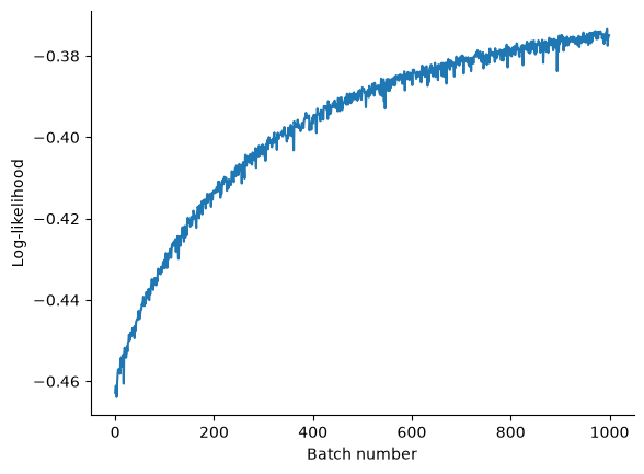
Plotting the resulting scores shows a similar curve as in previous sections using GLM.stochastic_fit:

fig, ax = plt.subplots()

ax.plot(scores)
ax.set_xlabel("Batch number")
ax.set_ylabel("Log-likelihood")

sns.despine(ax=ax)

../../_images/d1f2b11be52de1b2712a6aaccc00cdd8b50a81a99854712d4245700a4e70d5c0.png

Manual update loop for more control#

Set up the data and model#

Manual update loop calling GLM.update#

Manual update loop calling `GLM.update`#